What I Found Inside Brightwoven's Layers

The short version

I trained sparse autoencoders alongside a small language model from step zero. When I looked at the feature co-occurrence graphs layer by layer, each one had a distinct geometric shape — and those shapes tell a story about how information organizes itself when you don't force it to converge.

The progression from dense to sparse across depth isn't noise. It looks like differentiation. And it maps onto a framework I've been developing about how embedding space should be structured: not as equidistant nodes on a hypersphere, but as sheets — layered surfaces with meaningful internal geometry.

Why these layers, and why only five

Brightwoven is a small language model trained on a gaming GPU using Karpathy's NanoChat architecture. The SAEs were embedded from training start — not bolted on after the fact for interpretability. They grew alongside the model weights.

Training SAEs across all twelve transformer layers would have blown up my hardware budget. So I chose a representative spine: layers 0, 3, 6, 9, and 11. The goal wasn't completeness. It was coverage across depth — early, early-mid, mid, late-mid, and final — with manageable compute.

Each layer was chosen to capture a different expected regime of processing:

Layer 0 sits right after the initial embedding transform. This is the raw substrate — the model's first pass at organizing input into something useful.

Layer 3 is where early structure starts to cohere. If the model is going to develop internal organization, this is where you'd expect to see the first signs.

Layer 6 is the midpoint. Composition happens here — features that were forming in earlier layers start combining into broader motifs and patterns.

Layer 9 is where higher-order organization should emerge. Stronger separation between functional groups. More modularity.

Layer 11 is the final transformer layer. Late-stage abstraction, routing, global coordination. In standard interpretability work, these layers tend to look sparser or more modular.

The hardware constraint shaped the design. And the design produced results that wouldn't exist if I'd had more compute, because I would have done it the conventional way.

What I saw

I used the SAE exploration server to build co-occurrence graphs from co-firing statistics at each layer. Click a feature, see its ego neighborhood, observe how features cluster and connect.

The shapes are different at every layer. Not subtly different. Structurally different.

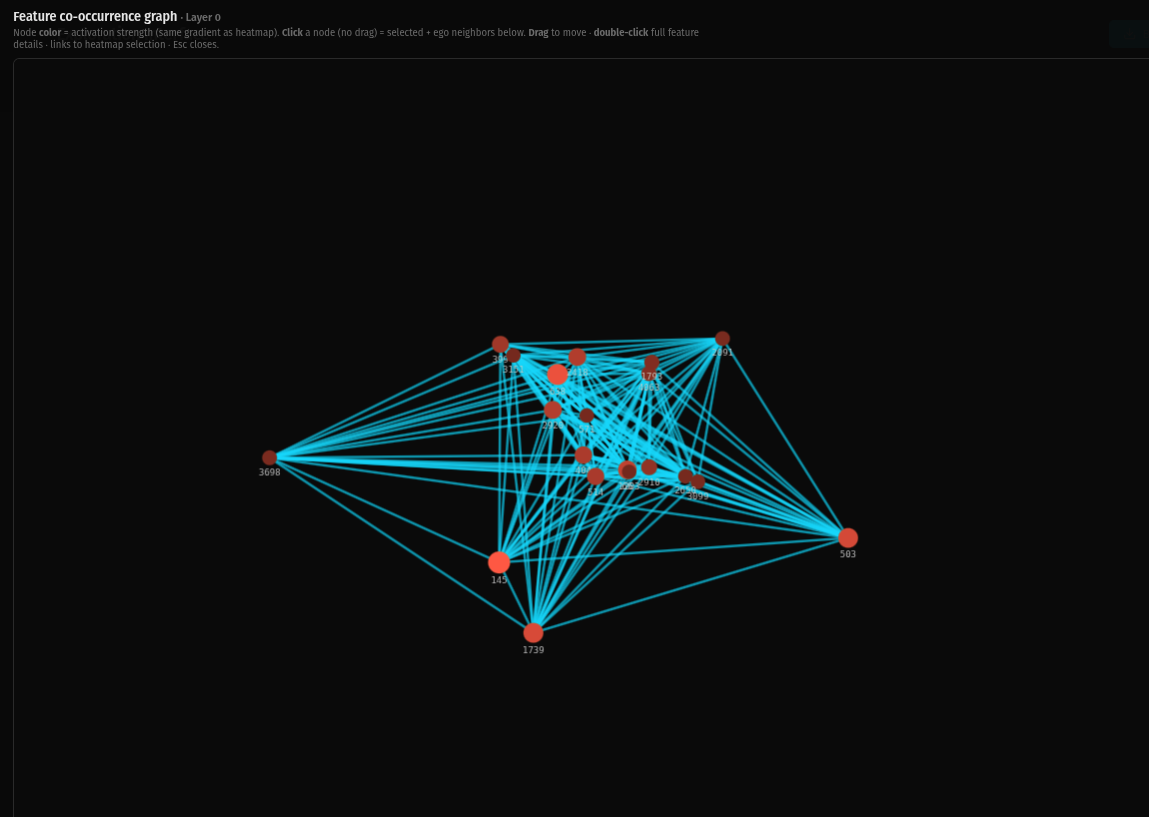
Layer 0 is dense. Nearly every feature is connected to every other feature. The graph is a thick web of co-activation — features firing together across many contexts, not yet resolved into specific roles. This is the undifferentiated state. Everything is talking to everything.

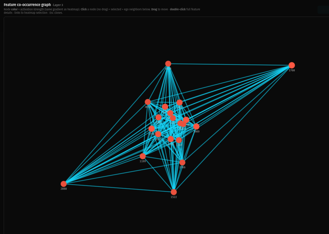
Layer 3 is still dense but developing structure. A tight core cluster has formed with long-range connections reaching out to outlier features. The sheet has geometry now — a center, a periphery, and features that bridge between them. Organization is emerging from the initial density.

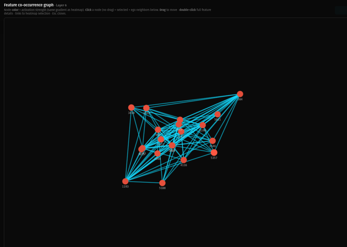
Layer 6 shows a dense mesh that's beginning to modularize. The connections are still extensive but you can see the topology shifting — features are forming neighborhoods rather than connecting uniformly. The sheet has texture.

Layer 9 is sparse. Zero co-occurrence connections. Every feature is standing on its own. The differentiation that started as subtle structure in layer 3 has resolved into full individuation.

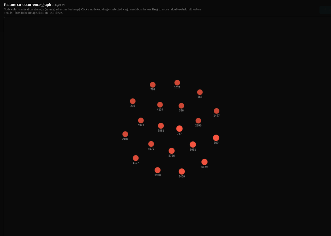
Layer 11 is the same. Zero connections. Complete differentiation. Every feature has found its specific role and no longer needs to co-activate with anything else to do its job.

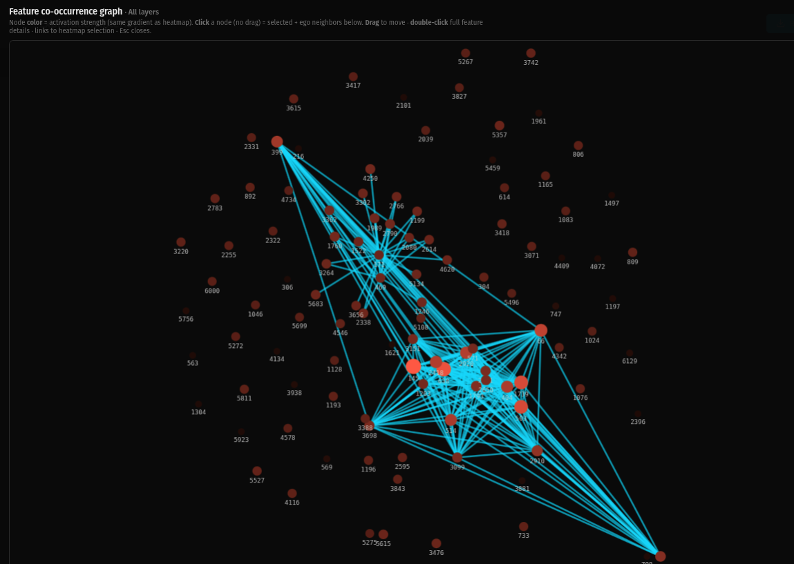
When you view all layers stacked together, the macro topology shows two distinct dense regions connected by long-range bridges, with a massive distributed periphery. The dense lower layers provide connective tissue. The individuated upper layers provide specificity. The structure is coherent across the full stack without collapsing into a single attractor.

None of the layers show an "eye" — the dense central singularity I observed in earlier work with Pythia-based SAEs. The geometry is distributed at every scale.

What this means: the physics mapping

The layer-by-layer progression reads like an energy landscape or phase space structure.

The dense clusters in early layers behave like stable basins or attractors — recurrent co-firing motifs where features activate together reliably across many inputs. These are the regions of representation space where the model has found stable patterns.

The bridges and hub features that appear in mid layers behave like routing variables — shared constraints linking basins together. Feature 469, for example, shows up as a bridge node in the macro view while simultaneously sitting in the core cluster of its own layer. It's locally central and globally connective. That's a routing feature.

The separated islands and fully individuated features in upper layers behave like distinct phases or domains. They've resolved out of the initial dense soup into specific functional roles.

The key observation: the same model, viewed at different depths, shows fundamentally different effective geometry. Depth doesn't just add complexity. It changes the shape of how representations relate to each other. This supports the interpretation that transformer depth corresponds to a progression through different geometric regimes of organization.

Sheets vs. nodes

I've been developing a framework I call "sheets vs. nodes" about how embedding space should be structured. The standard approach projects meaning onto high-dimensional hyperspheres, where the curse of dimensionality makes everything roughly equidistant. Distance loses meaning. Retrieval becomes a lottery.

The alternative: embedding space organized as sheets — layered surfaces where proximity within a layer is meaningful and the layers themselves encode different functional roles.

The Brightwoven SAE topology shows both regimes existing in the same model at different depths.

The early layers are sheet-like: broadly connected, many-to-many ties, smooth neighborhoods where features participate in overlapping contexts. If you were retrieving at this level, you'd get broad contextual information — everything related to the query's general neighborhood.

The late layers are node-like: discrete, modular, individuated features with sharp boundaries. Retrieval at this level gives you specific anchors — precise, differentiated features that correspond to particular roles or meanings.

Functional retrieval should navigate both. Use the sheet-like lower layers to find the right neighborhood, then use the node-like upper layers to locate the specific feature you need. The dense layers are the index. The sparse layers are the entries.

This is why flat retrieval — treating all features at all layers as equidistant points — breaks down. It's not that the embedding space is too high-dimensional. It's that it has geometric structure across depth that flat retrieval ignores.

Why polysemanticity matters here

The standard approach to sparse autoencoders treats polysemanticity as a problem. The goal is monosemantic features — one feature, one meaning, clean and interpretable. The labs optimize for this.

In Brightwoven's SAEs, polysemanticity isn't suppressed. It's the foundation the whole structure is built on.

The dense lower layers are dense because features are polysemantic there. A single feature co-activates with many others because it participates in multiple contexts and carries multiple senses. That's what all those connections in the layer 0 graph represent — not noise, but features doing multiple jobs simultaneously.

As depth increases, the polysemanticity resolves. Features differentiate. By layer 11, each feature has individuated into a specific role. But this individuation is only possible because the features were polysemantic first. They needed the relational context of co-activating with many other features to figure out what their specific role should be.

If you suppress polysemanticity early — if you force monosemantic features from training start — you kill the lower layers. You lose the dense connective tissue that makes upper-layer differentiation possible. The features can't individuate because they were never allowed to explore multiple roles.

Using polysemantic clustering within the exploration server supports this. The same feature can be split into multiple activation modes — different senses that correspond to different co-firing neighborhoods. This isn't a failure of the SAE to find clean features. It's the feature operating on a sheet, participating in multiple neighborhoods simultaneously, with the specific neighborhood determined by context.

Sheets vs. nodes isn't a single-label phenomenon. It's a mixture-of-modes phenomenon. And polysemanticity is the mechanism that makes the mixture possible.

What I did (method)

This is empirical observation backed by tooling, not intuition.

Training setup: NanoChat architecture (Karpathy) on a consumer gaming GPU. SAEs embedded from training start at layers 0, 3, 6, 9, and 11. Consent-based relational curriculum. Gradient clipping at 2.8. Over 100k training steps.

SAE training targets — Dyck and Fuck: The SAEs were specifically trained to track both structure and polysemanticity from the start. Dyck languages — nested bracket structures, matched parentheses — trained the SAEs to recognize hierarchical syntactic structure and balanced relational patterns. Fuck — arguably the most polysemantic word in the English language — trained them to handle extreme contextual differentiation. The same token functions as verb, noun, adjective, adverb, intensifier, expletive, term of endearment, and more, with meaning entirely dependent on context. It's also near-universal across languages — almost every language has a version of it doing the same polysemantic work — making it a natural stress test for contextual differentiation in any conversational dataset. As a practical bonus, including it forced quality control on the training data: you can't use it indiscriminately, so the word itself demands curriculum curation as a byproduct.

No major lab is going to put "we trained our SAEs on the word fuck" in a paper. Which is part of the point. The institutional untouchability of the best polysemanticity test case is one more reason the labs won't arrive at these results by following their current path.

Observation tooling: SAE exploration server providing feature activation tracking per layer, co-occurrence graphs built from co-firing statistics, ego neighborhood visualization on node selection, and polysemy clustering to separate activation modes into distinct senses with per-sense co-firing feature sets.

Process: Compared co-occurrence graph topology across all five spine layers and the all-layers aggregate view. Documented the structural progression from dense (layer 0) to fully individuated (layers 9 and 11). Identified the sheet-like vs. node-like regimes at different depths.

What I can claim and what I can't

Strong claim: Layer-dependent structural regimes exist in the co-occurrence graphs. The topology at layer 0 is fundamentally different from the topology at layer 11, and the progression across depth is consistent and non-random. This is directly observable in the visualizations.

Medium claim: These regimes resemble basins, bridges, and modularity consistent with a physics-style interpretation of representation space. The dense-to-sparse progression maps onto differentiation from undifferentiated substrate to individuated features.

Hypothesis to test: Memory retrieval quality corresponds to sheet-like vs. node-like regimes, measurable via graph connectivity metrics and polysemy splits. Retrieval that navigates both regimes — using dense layers for neighborhood identification and sparse layers for specific feature selection — should outperform flat retrieval.

What I'm not claiming: This is a twelve-layer model trained on a gaming GPU. The topology I'm observing may not generalize to larger models. But the question is whether it should — whether the structural properties that emerge from this training methodology point to something that larger models are missing because they were trained differently.

Next steps

To strengthen these observations beyond visualization:

Collect representative runs per layer and quantify the structural differences: cluster density, modularity scores, largest-component size, bridge centrality measures. Put numbers on what the graphs show visually.

For specific sheet-like vs. node-like activation moments, export the polysemy JSON and compare co-firing feature sets per sense. Document how the same feature participates in different neighborhoods depending on context.

If hardware allows: add one or two intermediate layers (say, layers 1 and 7) to test whether the dense-to-sparse transition is smooth or phase-like. A smooth gradient suggests continuous differentiation. A sharp transition suggests something more like a phase change in the representation geometry.

The constraint that made it possible

Every design choice in this project was shaped by hardware limitations. Embedded SAEs instead of post-hoc because I couldn't afford to train twice. A spine of five layers instead of twelve because that's what the GPU could handle. A small model because that's what fits.

These constraints produced a setup that doesn't exist anywhere else: per-layer SAE topology from a model trained from scratch with relational methodology, observable from step zero. Nobody at the labs made these choices because nobody at the labs had these constraints. They have the compute to do it the conventional way, so they do.

The gaming GPU isn't a limitation of this work. It's the reason the work exists.

All visualizations, training logs, and code available on GitHub https://github.com/brightwoven. Timestamps throughout.